Matlab-like Routines¶

The Matlab Module¶

matlab.py

MATLAB emulation functions.

This file contains a number of functions that emulate some of the functionality of MATLAB. The intent of these functions is to provide a simple interface to the python control systems library (python-control) for people who are familiar with the MATLAB Control Systems Toolbox (tm). Most of the functions are just calls to python-control functions defined elsewhere. Use ‘from control.matlab import *’ in python to include all of the functions defined here. Functions that are defined in other libraries that have the same names as their MATLAB equivalents are automatically imported here.

The following tables give an overview of the module control.matlab. They also show the implementation progress and the planned features of the module.

The symbols in the first column show the current state of a feature:

* : The feature is currently implemented.
- : The feature is not planned for implementation.
s : A similar feature from an other library (Scipy) is imported into the module, until the feature is implemented here.

Creating linear models¶

*	`tf()`	create transfer function (TF) models
	zpk	create zero/pole/gain (ZPK) models.
*	`ss()`	create state-space (SS) models
	dss	create descriptor state-space models
	delayss	create state-space models with delayed terms
	frd	create frequency response data (FRD) models
	lti/exp	create pure continuous-time delays (TF and ZPK only)
	filt	specify digital filters
-	lti/set	set/modify properties of LTI models
-	setdelaymodel	specify internal delay model (state space only)

Data extraction¶

	lti/tfdata	extract numerators and denominators
	lti/zpkdata	extract zero/pole/gain data
	lti/ssdata	extract state-space matrices
	lti/dssdata	descriptor version of SSDATA
	frd/frdata	extract frequency response data
	lti/get	access values of LTI model properties
	ss/getDelayModel	access internal delay model (state space)

Conversions¶

*	`tf()`	conversion to transfer function
	zpk	conversion to zero/pole/gain
*	`ss()`	conversion to state space
	frd	conversion to frequency data
	c2d	continuous to discrete conversion
	d2c	discrete to continuous conversion
	d2d	resample discrete-time model
	upsample	upsample discrete-time LTI systems
*	`ss2tf()`	state space to transfer function
s	ss2zpk	transfer function to zero-pole-gain
*	`tf2ss()`	transfer function to state space
s	tf2zpk	transfer function to zero-pole-gain
s	zpk2ss	zero-pole-gain to state space
s	zpk2tf	zero-pole-gain to transfer function

System interconnections¶

	append	group LTI models by appending inputs/outputs
*	`parallel()`	connect LTI models in parallel (see also overloaded `+`)
*	`series()`	connect LTI models in series (see also overloaded `*`)
*	`feedback()`	connect lti models with a feedback loop
	lti/lft	generalized feedback interconnection
	lti/connect	arbitrary interconnection of lti models
	sumblk	summing junction (for use with connect)
	strseq	builds sequence of indexed strings (for I/O naming)

System gain and dynamics¶

*	`dcgain()`	steady-state (D.C.) gain
	lti/bandwidth	system bandwidth
	lti/norm	h2 and Hinfinity norms of LTI models
*	`pole()`	system poles
*	`zero()`	system (transmission) zeros
	lti/order	model order (number of states)
*	`pzmap()`	pole-zero map (TF only)
	lti/iopzmap	input/output pole-zero map
	damp	natural frequency, damping of system poles
	esort	sort continuous poles by real part
	dsort	sort discrete poles by magnitude
	lti/stabsep	stable/unstable decomposition
	lti/modsep	region-based modal decomposition

Time-domain analysis¶

*	`step()`	step response
	stepinfo	step response characteristics
*	`impulse()`	impulse response
*	`initial()`	free response with initial conditions
*	`lsim()`	response to user-defined input signal
	lsiminfo	linear response characteristics
	gensig	generate input signal for LSIM
	covar	covariance of response to white noise

Frequency-domain analysis¶

*	`bode()`	Bode plot of the frequency response
	lti/bodemag	Bode magnitude diagram only
	sigma	singular value frequency plot
*	`nyquist()`	Nyquist plot
*	`nichols()`	Nichols plot
*	`margin()`	gain and phase margins
	lti/allmargin	all crossover frequencies and margins
*	`freqresp()`	frequency response over a frequency grid
*	`evalfr()`	frequency response at single frequency

Model simplification¶

	minreal	minimal realization; pole/zero cancellation
	ss/sminreal	structurally minimal realization
*	`hsvd()`	hankel singular values (state contributions)
*	`balred()`	reduced-order approximations of LTI models
*	`modred()`	model order reduction

Compensator design¶

*	`rlocus()`	evans root locus
*	`place()`	pole placement
	estim	form estimator given estimator gain
	reg	form regulator given state-feedback and estimator gains

LQR/LQG design¶

	ss/lqg	single-step LQG design
*	`lqr()`	linear quadratic (LQ) state-fbk regulator
	dlqr	discrete-time LQ state-feedback regulator
	lqry	LQ regulator with output weighting
	lqrd	discrete LQ regulator for continuous plant
	ss/lqi	Linear-Quadratic-Integral (LQI) controller
	ss/kalman	Kalman state estimator
	ss/kalmd	discrete Kalman estimator for cts plant
	ss/lqgreg	build LQG regulator from LQ gain and Kalman estimator
	ss/lqgtrack	build LQG servo-controller
	augstate	augment output by appending states

State-space (SS) models¶

*	`rss()`	random stable cts-time state-space models
*	`drss()`	random stable disc-time state-space models
	ss2ss	state coordinate transformation
	canon	canonical forms of state-space models
*	`ctrb()`	controllability matrix
*	`obsv()`	observability matrix
*	`gram()`	controllability and observability gramians
	ss/prescale	optimal scaling of state-space models.
	balreal	gramian-based input/output balancing
	ss/xperm	reorder states.

Frequency response data (FRD) models¶

	frd/chgunits	change frequency vector units
	frd/fcat	merge frequency responses
	frd/fselect	select frequency range or subgrid
	frd/fnorm	peak gain as a function of frequency
	frd/abs	entrywise magnitude of frequency response
	frd/real	real part of the frequency response
	frd/imag	imaginary part of the frequency response
	frd/interp	interpolate frequency response data
	mag2db	convert magnitude to decibels (dB)
	db2mag	convert decibels (dB) to magnitude

Time delays¶

	lti/hasdelay	true for models with time delays
	lti/totaldelay	total delay between each input/output pair
	lti/delay2z	replace delays by poles at z=0 or FRD phase shift
*	`pade()`	pade approximation of time delays

Model dimensions and characteristics¶

	class	model type (‘tf’, ‘zpk’, ‘ss’, or ‘frd’)
	isa	test if model is of given type
	tf/size	model sizes
	lti/ndims	number of dimensions
	lti/isempty	true for empty models
	lti/isct	true for continuous-time models
	lti/isdt	true for discrete-time models
	lti/isproper	true for proper models
	lti/issiso	true for single-input/single-output models
	lti/isstable	true for models with stable dynamics
	lti/reshape	reshape array of linear models

Overloaded arithmetic operations¶

*	+ and -	add, subtract systems (parallel connection)
*	*	multiply systems (series connection)
	/	right divide – sys1*inv(sys2)
-	\	left divide – inv(sys1)*sys2
	^	powers of a given system
	‘	pertransposition
	.’	transposition of input/output map
	.*	element-by-element multiplication
	[..]	concatenate models along inputs or outputs
	lti/stack	stack models/arrays along some dimension
	lti/inv	inverse of an LTI system
	lti/conj	complex conjugation of model coefficients

Matrix equation solvers and linear algebra¶

*	`lyap()`	solve continuous-time Lyapunov equations
*	`dlyap()`	solve discrete-time Lyapunov equations
	lyapchol, dlyapchol	square-root Lyapunov solvers
*	`care()`	solve continuous-time algebraic Riccati equations
*	`dare()`	solve disc-time algebraic Riccati equations
	gcare, gdare	generalized Riccati solvers
	bdschur	block diagonalization of a square matrix

Additional functions¶

*	`gangof4()`	generate the Gang of 4 sensitivity plots
*	`linspace()`	generate a set of numbers that are linearly spaced
*	`logspace()`	generate a set of numbers that are logarithmically spaced
*	`unwrap()`	unwrap phase angle to give continuous curve

matlab.bode(*args, **keywords)¶

Bode plot of the frequency response

Examples

>>> sys = ss("1. -2; 3. -4", "5.; 7", "6. 8", "9.") 
>>> mag, phase, omega = bode(sys)

Todo

Document these use cases

```
>>> bode(sys, w)
```
```
>>> bode(sys1, sys2, ..., sysN)
```
```
>>> bode(sys1, sys2, ..., sysN, w)
```

>>> bode(sys1, 'plotstyle1', ..., sysN, 'plotstyleN')

matlab.dcgain(*args)¶

Compute the gain of the system in steady state.

The function takes either 1, 2, 3, or 4 parameters:

Parameters :

A, B, C, D: array-like :

A linear system in state space form.

Z, P, k: array-like, array-like, number :

A linear system in zero, pole, gain form.

num, den: array-like :

A linear system in transfer function form.

sys: Lti (StateSpace or TransferFunction) :

A linear system object.

Returns :

gain: matrix :

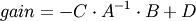
The gain of each output versus each input: $y = gain \cdot u$

Notes

This function is only useful for systems with invertible system matrix A.

All systems are first converted to state space form. The function then computes:

$gain = - C \cdot A^{-1} \cdot B + D$

matlab.drss(states=1, inputs=1, outputs=1)¶

Create a stable discrete random state space object.

Parameters :

states: integer :

Number of state variables

inputs: integer :

Number of system inputs

outputs: integer :

Number of system outputs

Returns :

sys: StateSpace :

The randomly created linear system

Raises :

ValueError :

if any input is not a positive integer

See also

rss

Notes

If the number of states, inputs, or outputs is not specified, then the missing numbers are assumed to be 1. The poles of the returned system will always have a magnitude less than 1.

matlab.evalfr(sys, omega)¶

Evaluate the transfer function of an LTI system at an angular frequency.

Parameters :

sys: StateSpace or TransferFunction :

Linear system

omega: scalar :

Frequency

Returns :

fresp: ndarray :

See also

freqresp, bode

Notes

This function is a wrapper for StateSpace.evalfr and TransferFunction.evalfr.

Examples

>>> sys = ss("1. -2; 3. -4", "5.; 7", "6. 8", "9.")
>>> evalfr(sys, 1.)
array([[ 44.8-21.4j]])
>>> # This is the transfer function matrix evaluated at s = i.

Todo

Add example with MIMO system

matlab.freqresp(sys, omega)¶

Frequency response of an LTI system at multiple angular frequencies.

Parameters :

sys: StateSpace or TransferFunction :

Linear system

omega: array_like :

List of frequencies

Returns :

mag: ndarray :

phase: ndarray :

omega: list, tuple, or ndarray :

See also

evalfr, bode

Notes

This function is a wrapper for StateSpace.freqresp and TransferFunction.freqresp. The output omega is a sorted version of the input omega.

Examples

>>> sys = ss("1. -2; 3. -4", "5.; 7", "6. 8", "9.")
>>> mag, phase, omega = freqresp(sys, [0.1, 1., 10.])
>>> mag
array([[[ 58.8576682 ,  49.64876635,  13.40825927]]])
>>> phase
array([[[-0.05408304, -0.44563154, -0.66837155]]])

Todo

Add example with MIMO system

#>>> sys = rss(3, 2, 2) #>>> mag, phase, omega = freqresp(sys, [0.1, 1., 10.]) #>>> mag[0, 1, :] #array([ 55.43747231, 42.47766549, 1.97225895]) #>>> phase[1, 0, :] #array([-0.12611087, -1.14294316, 2.5764547 ]) #>>> # This is the magnitude of the frequency response from the 2nd #>>> # input to the 1st output, and the phase (in radians) of the #>>> # frequency response from the 1st input to the 2nd output, for #>>> # s = 0.1i, i, 10i.

matlab.impulse(sys, T=None, input=0, output=0, **keywords)¶

Impulse response of a linear system

If the system has multiple inputs or outputs (MIMO), one input and one output must be selected for the simulation. The parameters input and output do this. All other inputs are set to 0, all other outputs are ignored.

Parameters :

sys: StateSpace, TransferFunction :

LTI system to simulate

T: array-like object, optional :

Time vector (argument is autocomputed if not given)

input: int :

Index of the input that will be used in this simulation.

output: int :

Index of the output that will be used in this simulation.

**keywords: :

Additional keyword arguments control the solution algorithm for the differential equations. These arguments are passed on to the function lsim(), which in turn passes them on to scipy.integrate.odeint(). See the documentation for scipy.integrate.odeint() for information about these arguments.

Returns :

yout: array :

Response of the system

T: array :

Time values of the output

See also

lsim, step, initial

Examples

>>> T, yout = impulse(sys, T) 

matlab.initial(sys, T=None, X0=0.0, input=0, output=0, **keywords)¶

Initial condition response of a linear system

If the system has multiple inputs or outputs (MIMO), one input and one output have to be selected for the simulation. The parameters input and output do this. All other inputs are set to 0, all other outputs are ignored.

Parameters :

sys: StateSpace, or TransferFunction :

LTI system to simulate

T: array-like object, optional :

Time vector (argument is autocomputed if not given)

X0: array-like object or number, optional :

Initial condition (default = 0)

Numbers are converted to constant arrays with the correct shape.

input: int :

Index of the input that will be used in this simulation.

output: int :

Index of the output that will be used in this simulation.

**keywords: :

Additional keyword arguments control the solution algorithm for the differential equations. These arguments are passed on to the function lsim(), which in turn passes them on to scipy.integrate.odeint(). See the documentation for scipy.integrate.odeint() for information about these arguments.

Returns :

yout: array :

Response of the system

T: array :

Time values of the output

See also

lsim, step, impulse

Examples

>>> T, yout = initial(sys, T, X0)

matlab.lsim(sys, U=0.0, T=None, X0=0.0, **keywords)¶

Simulate the output of a linear system.

As a convenience for parameters U, X0: Numbers (scalars) are converted to constant arrays with the correct shape. The correct shape is inferred from arguments sys and T.

Parameters :

sys: Lti (StateSpace, or TransferFunction) :

LTI system to simulate

U: array-like or number, optional :

Input array giving input at each time T (default = 0).

If U is None or 0, a special algorithm is used. This special algorithm is faster than the general algorithm, which is used otherwise.

T: array-like :

Time steps at which the input is defined, numbers must be (strictly monotonic) increasing.

X0: array-like or number, optional :

Initial condition (default = 0).

**keywords: :

Additional keyword arguments control the solution algorithm for the differential equations. These arguments are passed on to the function scipy.integrate.odeint(). See the documentation for scipy.integrate.odeint() for information about these arguments.

Returns :

yout: array :

Response of the system.

T: array :

Time values of the output.

xout: array :

Time evolution of the state vector.

See also

step, initial, impulse

Examples

>>> T, yout, xout = lsim(sys, U, T, X0)

matlab.margin(*args)¶

Calculate gain and phase margins and associated crossover frequencies

Function margin takes either 1 or 3 parameters.

Parameters :

sys : StateSpace or TransferFunction

Linear SISO system

mag, phase, w : array_like

Input magnitude, phase (in deg.), and frequencies (rad/sec) from bode frequency response data

Returns :

gm, pm, wg, wp : float

Gain margin gm, phase margin pm (in deg), and associated crossover frequencies wg and wp (in rad/sec) of SISO open-loop. If more than one crossover frequency is detected, returns the lowest corresponding margin.

Examples

>>> sys = ss("1. -2; 3. -4", "5.; 7", "6. 8", "9.")
>>> gm, pm, wg, wp = margin(sys)
margin: no magnitude crossings found

Todo

better ecample system!

#>>> gm, pm, wg, wp = margin(mag, phase, w)

matlab.ngrid()¶

Nichols chart grid

Parameters :

cl_mags : array-like (dB), optional

Array of closed-loop magnitudes defining the iso-gain lines on a custom Nichols chart.

cl_phases : array-like (degrees), optional

Array of closed-loop phases defining the iso-phase lines on a custom Nichols chart. Must be in the range -360 < cl_phases < 0

matlab.pole(sys)¶

Compute system poles.

Parameters :

sys: StateSpace or TransferFunction :

Linear system

Returns :

poles: ndarray :

Array that contains the system’s poles.

Raises :

NotImplementedError :

when called on a TransferFunction object

See also

zero

Notes

This function is a wrapper for StateSpace.pole and TransferFunction.pole.

matlab.rlocus(sys, klist=None, **keywords)¶

Root locus plot

Parameters :

sys: StateSpace or TransferFunction :

Linear system

klist: :

optional list of gains

Returns :

rlist: :

list of roots for each gain

klist: :

list of gains used to compute roots

matlab.rss(states=1, inputs=1, outputs=1)¶

Create a stable continuous random state space object.

Parameters :

states: integer :

Number of state variables

inputs: integer :

Number of system inputs

outputs: integer :

Number of system outputs

Returns :

sys: StateSpace :

The randomly created linear system

Raises :

ValueError :

if any input is not a positive integer

See also

drss

Notes

If the number of states, inputs, or outputs is not specified, then the missing numbers are assumed to be 1. The poles of the returned system will always have a negative real part.

matlab.ss(*args)¶

Create a state space system.

The function accepts either 1 or 4 parameters:

ss(sys)

Convert a linear system into space system form. Always creates a new system, even if sys is already a StateSpace object.

ss(A, B, C, D)

Create a state space system from the matrices of its state and output equations:

$\dot x = A \cdot x + B \cdot u y = C \cdot x + D \cdot u$

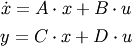
The matrices can be given as array like data types or strings. Everything that the constructor of numpy.matrix accepts is permissible here too.

Parameters :

sys: Lti (StateSpace or TransferFunction) :

A linear system

A: array_like or string :

System matrix

B: array_like or string :

Control matrix

C: array_like or string :

Output matrix

D: array_like or string :

Feed forward matrix

Returns :

out: StateSpace :

The new linear system

Raises :

ValueError :

if matrix sizes are not self-consistent

See also

tf, ss2tf, tf2ss

Examples

>>> # Create a StateSpace object from four "matrices".
>>> sys1 = ss("1. -2; 3. -4", "5.; 7", "6. 8", "9.") 

>>> # Convert a TransferFunction to a StateSpace object.
>>> sys_tf = tf([2.], [1., 3])
>>> sys2 = ss(sys_tf) 

matlab.ss2tf(*args)¶

Transform a state space system to a transfer function.

The function accepts either 1 or 4 parameters:

ss2tf(sys)

Convert a linear system into space system form. Always creates a new system, even if sys is already a StateSpace object.

ss2tf(A, B, C, D)

Create a state space system from the matrices of its state and output equations.

For details see: ss()

Parameters :

sys: StateSpace :

A linear system

A: array_like or string :

System matrix

B: array_like or string :

Control matrix

C: array_like or string :

Output matrix

D: array_like or string :

Feed forward matrix

Returns :

out: TransferFunction :

New linear system in transfer function form

Raises :

ValueError :

if matrix sizes are not self-consistent, or if an invalid number of arguments is passed in

TypeError :

if sys is not a StateSpace object

See also

tf, ss, tf2ss

Examples

>>> A = [[1., -2], [3, -4]]
>>> B = [[5.], [7]]
>>> C = [[6., 8]]
>>> D = [[9.]]
>>> sys1 = ss2tf(A, B, C, D)

>>> sys_ss = ss(A, B, C, D)
>>> sys2 = ss2tf(sys_ss) 

matlab.step(sys, T=None, X0=0.0, input=0, output=0, **keywords)¶

Step response of a linear system

If the system has multiple inputs or outputs (MIMO), one input and one output have to be selected for the simulation. The parameters input and output do this. All other inputs are set to 0, all other outputs are ignored.

Parameters :

sys: StateSpace, or TransferFunction :

LTI system to simulate

T: array-like object, optional :

Time vector (argument is autocomputed if not given)

X0: array-like or number, optional :

Initial condition (default = 0)

Numbers are converted to constant arrays with the correct shape.

input: int :

Index of the input that will be used in this simulation.

output: int :

Index of the output that will be used in this simulation.

**keywords: :

Additional keyword arguments control the solution algorithm for the differential equations. These arguments are passed on to the function control.forced_response(), which in turn passes them on to scipy.integrate.odeint(). See the documentation for scipy.integrate.odeint() for information about these arguments.

Returns :

yout: array :

Response of the system

T: array :

Time values of the output

See also

lsim, initial, impulse

Examples

>>> T, yout = step(sys, T, X0)

matlab.tf(*args)¶

Create a transfer function system. Can create MIMO systems.

The function accepts either 1 or 2 parameters:

tf(sys)

Convert a linear system into transfer function form. Always creates a new system, even if sys is already a TransferFunction object.

tf(num, den)

Create a transfer function system from its numerator and denominator polynomial coefficients.

If num and den are 1D array_like objects, the function creates a SISO system.

To create a MIMO system, num and den need to be 2D nested lists of array_like objects. (A 3 dimensional data structure in total.) (For details see note below.)

Parameters :

sys: Lti (StateSpace or TransferFunction) :

A linear system

num: array_like, or list of list of array_like :

Polynomial coefficients of the numerator

den: array_like, or list of list of array_like :

Polynomial coefficients of the denominator

Returns :

out: TransferFunction :

The new linear system

Raises :

ValueError :

if num and den have invalid or unequal dimensions

TypeError :

if num or den are of incorrect type

See also

ss, ss2tf, tf2ss

Notes

Todo

The next paragraph contradicts the comment in the example! Also “input” should come before “output” in the sentence:

“from the (j+1)st output to the (i+1)st input”

num[i][j] contains the polynomial coefficients of the numerator for the transfer function from the (j+1)st output to the (i+1)st input. den[i][j] works the same way.

The coefficients [2, 3, 4] denote the polynomial $2 \cdot s^2 + 3 \cdot s + 4$ .

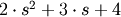Examples

>>> # Create a MIMO transfer function object
>>> # The transfer function from the 2nd input to the 1st output is
>>> # (3s + 4) / (6s^2 + 5s + 4).
>>> num = [[[1., 2.], [3., 4.]], [[5., 6.], [7., 8.]]]
>>> den = [[[9., 8., 7.], [6., 5., 4.]], [[3., 2., 1.], [-1., -2., -3.]]]
>>> sys1 = tf(num, den)

>>> # Convert a StateSpace to a TransferFunction object.
>>> sys_ss = ss("1. -2; 3. -4", "5.; 7", "6. 8", "9.")
>>> sys2 = tf(sys1) 

matlab.tf2ss(*args)¶

Transform a transfer function to a state space system.

The function accepts either 1 or 2 parameters:

tf2ss(sys)

Convert a linear system into transfer function form. Always creates a new system, even if sys is already a TransferFunction object.

tf2ss(num, den)

Create a transfer function system from its numerator and denominator polynomial coefficients.

For details see: tf()

Parameters :

sys: Lti (StateSpace or TransferFunction) :

A linear system

num: array_like, or list of list of array_like :

Polynomial coefficients of the numerator

den: array_like, or list of list of array_like :

Polynomial coefficients of the denominator

Returns :

out: StateSpace :

New linear system in state space form

Raises :

ValueError :

if num and den have invalid or unequal dimensions, or if an invalid number of arguments is passed in

TypeError :

if num or den are of incorrect type, or if sys is not a TransferFunction object

See also

ss, tf, ss2tf

Examples

>>> num = [[[1., 2.], [3., 4.]], [[5., 6.], [7., 8.]]]
>>> den = [[[9., 8., 7.], [6., 5., 4.]], [[3., 2., 1.], [-1., -2., -3.]]]
>>> sys1 = tf2ss(num, den)

>>> sys_tf = tf(num, den)
>>> sys2 = tf2ss(sys_tf) 

matlab.zero(sys)¶

Compute system zeros.

Parameters :

sys: StateSpace or TransferFunction :

Linear system

Returns :

zeros: ndarray :

Array that contains the system’s zeros.

Raises :

NotImplementedError :

when called on a TransferFunction object or a MIMO StateSpace object

See also

pole

Notes

This function is a wrapper for StateSpace.zero and TransferFunction.zero.

Todo

The following functions should be documented in their own modules! This is only a temporary solution.

pzmap.pzmap(sys, Plot=True, title='Pole Zero Map')¶

Plot a pole/zero map for a linear system.

Parameters :

sys: Lti (StateSpace or TransferFunction) :

Linear system for which poles and zeros are computed.

Plot: bool :

If True a graph is generated with Matplotlib, otherwise the poles and zeros are only computed and returned.

Returns :

pole: array :

The systems poles

zeros: array :

The system’s zeros.

freqplot.nyquist(syslist, omega=None, Plot=True)¶

Nyquist plot for a system

Plots a Nyquist plot for the system over a (optional) frequency range.

Parameters :

syslist : list of Lti

List of linear input/output systems (single system is OK)

omega : freq_range

Range of frequencies (list or bounds) in rad/sec

Plot : boolean

if True, plot magnitude

Returns :

real : array

real part of the frequency response array

imag : array

imaginary part of the frequency response array

freq : array

frequencies

Examples

>>> from matlab import ss
>>> sys = ss("1. -2; 3. -4", "5.; 7", "6. 8", "9.")
>>> real, imag, freq = nyquist(sys)

nichols.nichols(syslist, omega=None, grid=True)¶

Nichols plot for a system

Plots a Nichols plot for the system over a (optional) frequency range.

Parameters :

syslist : list of Lti, or Lti

List of linear input/output systems (single system is OK)

omega : array_like

Range of frequencies (list or bounds) in rad/sec

grid : boolean, optional

True if the plot should include a Nichols-chart grid. Default is True.

Returns :

None :

statefbk.place(A, B, p)¶

Place closed loop eigenvalues

Parameters :

A : 2-d array

Dynamics matrix

B : 2-d array

Input matrix

p : 1-d list

Desired eigenvalue locations

Returns :

K : 2-d array

Gains such that A - B K has given eigenvalues

Examples

>>> A = [[-1, -1], [0, 1]]
>>> B = [[0], [1]]
>>> K = place(A, B, [-2, -5])

statefbk.lqr(*args, **keywords)¶

Linear quadratic regulator design

The lqr() function computes the optimal state feedback controller that minimizes the quadratic cost

$J = \int_0^\infty x' Q x + u' R u + 2 x' N u$

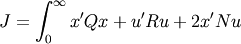
The function can be called with either 3, 4, or 5 arguments:

lqr(sys, Q, R)
lqr(sys, Q, R, N)
lqr(A, B, Q, R)
lqr(A, B, Q, R, N)

Parameters :

A, B: 2-d array :

Dynamics and input matrices

sys: Lti (StateSpace or TransferFunction) :

Linear I/O system

Q, R: 2-d array :

State and input weight matrices

N: 2-d array, optional :

Cross weight matrix

Returns :

K: 2-d array :

State feedback gains

S: 2-d array :

Solution to Riccati equation

E: 1-d array :

Eigenvalues of the closed loop system

Examples

>>> K, S, E = lqr(sys, Q, R, [N])
>>> K, S, E = lqr(A, B, Q, R, [N])

statefbk.ctrb(A, B)¶

Controllabilty matrix

Parameters :

A, B: array_like or string :

Dynamics and input matrix of the system

Returns :

C: matrix :

Controllability matrix

Examples

>>> C = ctrb(A, B)

statefbk.obsv(A, C)¶

Observability matrix

Parameters :

A, C: array_like or string :

Dynamics and output matrix of the system

Returns :

O: matrix :

Observability matrix

Examples

>>> O = obsv(A, C)

statefbk.gram(sys, type)¶

Gramian (controllability or observability)

Parameters :

sys: StateSpace :

State-space system to compute Gramian for

type: String :

Type of desired computation. type is either ‘c’ (controllability) or ‘o’ (observability).

Returns :

gram: array :

Gramian of system

Raises :

ValueError :

if system is not instance of StateSpace class

if type is not ‘c’ or ‘o’

if system is unstable (sys.A has eigenvalues not in left half plane)

ImportError :

if slycot routin sb03md cannot be found

Examples

>>> Wc = gram(sys,'c')
>>> Wo = gram(sys,'o')

delay.pade(T, n=1)¶

Create a linear system that approximates a delay.

Return the numerator and denominator coefficients of the Pade approximation.

Parameters :

T : number

time delay

n : integer

order of approximation

Returns :

num, den : array

Polynomial coefficients of the delay model, in descending powers of s.

Notes

Based on an algorithm in Golub and van Loan, “Matrix Computation” 3rd. Ed. pp. 572-574.

freqplot.gangof4(P, C, omega=None)¶

Plot the “Gang of 4” transfer functions for a system

Generates a 2x2 plot showing the “Gang of 4” sensitivity functions [T, PS; CS, S]

Parameters :

P, C : Lti

Linear input/output systems (process and control)

omega : array

Range of frequencies (list or bounds) in rad/sec

Returns :

None :

ctrlutil.unwrap(angle, period=6.2831853071795862)¶

Unwrap a phase angle to give a continuous curve

Parameters :

X : array_like

Input array

period : number

Input period (usually either 2``*``pi or 360)

Returns :

Y : array_like

Output array, with jumps of period/2 eliminated

Examples

>>> import numpy as np
>>> X = [5.74, 5.97, 6.19, 0.13, 0.35, 0.57]
>>> unwrap(X, period=2 * np.pi)
[5.74, 5.97, 6.19, 6.413185307179586, 6.633185307179586, 6.8531853071795865]

mateqn.lyap(A, Q, C=None, E=None)¶

X = lyap(A,Q) solves the continuous-time Lyapunov equation

A X + X A^T + Q = 0

where A and Q are square matrices of the same dimension. Further, Q must be symmetric.

X = lyap(A,Q,C) solves the Sylvester equation

A X + X Q + C = 0

where A and Q are square matrices.

X = lyap(A,Q,None,E) solves the generalized continuous-time Lyapunov equation

A X E^T + E X A^T + Q = 0

where Q is a symmetric matrix and A, Q and E are square matrices of the same dimension.

mateqn.dlyap(A, Q, C=None, E=None)¶

dlyap(A,Q) solves the discrete-time Lyapunov equation

A X A^T - X + Q = 0

where A and Q are square matrices of the same dimension. Further Q must be symmetric.

dlyap(A,Q,C) solves the Sylvester equation

A X Q^T - X + C = 0

where A and Q are square matrices.

dlyap(A,Q,None,E) solves the generalized discrete-time Lyapunov equation

A X A^T - E X E^T + Q = 0

where Q is a symmetric matrix and A, Q and E are square matrices of the same dimension.

mateqn.care(A, B, Q, R=None, S=None, E=None)¶

(X,L,G) = care(A,B,Q) solves the continuous-time algebraic Riccati equation

A^T X + X A - X B B^T X + Q = 0

where A and Q are square matrices of the same dimension. Further, Q is a symmetric matrix. The function returns the solution X, the gain matrix G = B^T X and the closed loop eigenvalues L, i.e., the eigenvalues of A - B G.

(X,L,G) = care(A,B,Q,R,S,E) solves the generalized continuous-time algebraic Riccati equation

A^T X E + E^T X A - (E^T X B + S) R^-1 (B^T X E + S^T) + Q = 0

where A, Q and E are square matrices of the same dimension. Further, Q and R are symmetric matrices. The function returns the solution X, the gain matrix G = R^-1 (B^T X E + S^T) and the closed loop eigenvalues L, i.e., the eigenvalues of A - B G , E.

mateqn.dare(A, B, Q, R, S=None, E=None)¶

(X,L,G) = dare(A,B,Q,R) solves the discrete-time algebraic Riccati equation

A^T X A - X - A^T X B (B^T X B + R)^-1 B^T X A + Q = 0

where A and Q are square matrices of the same dimension. Further, Q is a symmetric matrix. The function returns the solution X, the gain matrix G = (B^T X B + R)^-1 B^T X A and the closed loop eigenvalues L, i.e., the eigenvalues of A - B G.

(X,L,G) = dare(A,B,Q,R,S,E) solves the generalized discrete-time algebraic Riccati equation

A^T X A - E^T X E - (A^T X B + S) (B^T X B + R)^-1 (B^T X A + S^T) +

Q = 0

where A, Q and E are square matrices of the same dimension. Further, Q and R are symmetric matrices. The function returns the solution X, the gain matrix G = (B^T X B + R)^-1 (B^T X A + S^T) and the closed loop eigenvalues L, i.e., the eigenvalues of A - B G , E.

Matlab-like Routines¶

The Matlab Module¶

Creating linear models¶

Data extraction¶

Conversions¶

System interconnections¶

System gain and dynamics¶

Time-domain analysis¶

Frequency-domain analysis¶

Model simplification¶

Compensator design¶

LQR/LQG design¶

State-space (SS) models¶

Frequency response data (FRD) models¶

Time delays¶

Model dimensions and characteristics¶

Overloaded arithmetic operations¶

Matrix equation solvers and linear algebra¶

Additional functions¶

Table Of Contents

Previous topic

Next topic

This Page

Navigation

Matlab-like Routines¶

The Matlab Module¶

Creating linear models¶

Data extraction¶

Conversions¶

System interconnections¶

System gain and dynamics¶

Time-domain analysis¶

Frequency-domain analysis¶

Model simplification¶

Compensator design¶

LQR/LQG design¶

State-space (SS) models¶

Frequency response data (FRD) models¶

Time delays¶

Model dimensions and characteristics¶

Overloaded arithmetic operations¶

Matrix equation solvers and linear algebra¶

Additional functions¶

Table Of Contents

Previous topic

Next topic

This Page

Quick search

Navigation